Find cell values easily using Excel's Lookup Wizard
Rather than scrolling through long tables of data in a worksheet, let this wizard find the value you're looking for automatically.


Microsoft Excel can handle data tables with hundreds or even thousands of rows and columns. That's great, unless you're trying to find a specific cell's value, which could have you scrolling up and down, left and right looking for that needle of data in a haystack of cells. If your table is formatted correctly, you can use Excel's Lookup Wizard to display the data in a cell automatically.
To see if you have the Lookup Wizard installed in Excel 2003, click Tools and look for a Lookup option, probably at the bottom of the menu. In Excel 2007, click the Formulas tab and look to the far right for a Lookup option in the Solutions section of the ribbon. If the wizard isn't there, load it in Excel 2003 by clicking Tools > Add-Ins > Lookup Wizard > OK > Yes, or in Excel 2007 by selecting the Office button, and clicking Excel Options > Add-Ins > Lookup Wizard > Go > Lookup Wizard > OK > Yes. You may be asked to insert your Office install CD to complete the installation. When the dialog box closes, you should have a Lookup option on your Tools menu in Excel 2003, or a Lookup button in the Solutions section at the far right under Excel 2007's Formulas tab.
Note that your table can't have any empty cells, and it must have headings. (Additionally, if you use the wizard to find a range of values, the rows must be sorted; see below for more on searching for value ranges.)
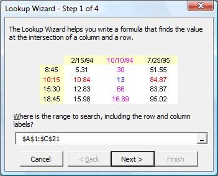
To find a cell's data, select the cell range you want to search, including the table headers, and click Tools > Lookup in Excel 2003, or click the aforementioned Lookup button in the Solutions area under the Formulas tab in Excel 2007. In step 1 of the 4-step wizard, verify that the range is correct, and click Next.
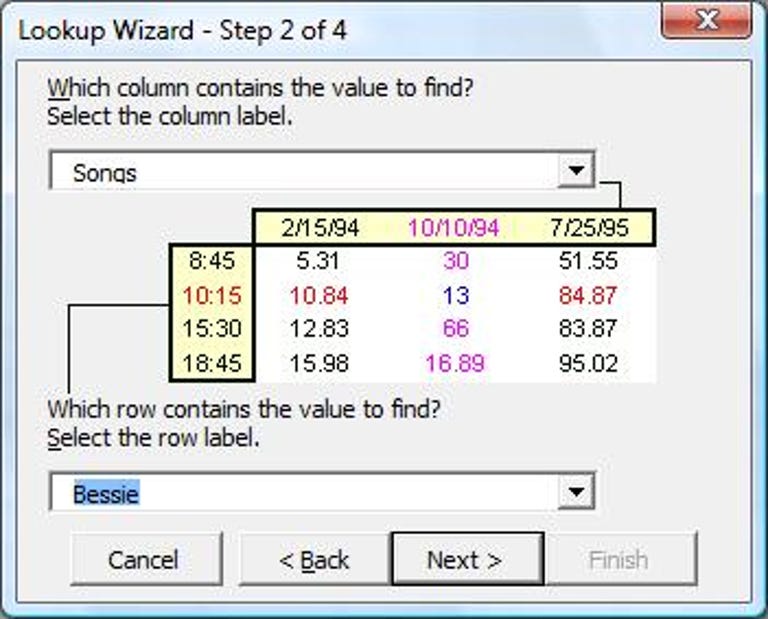
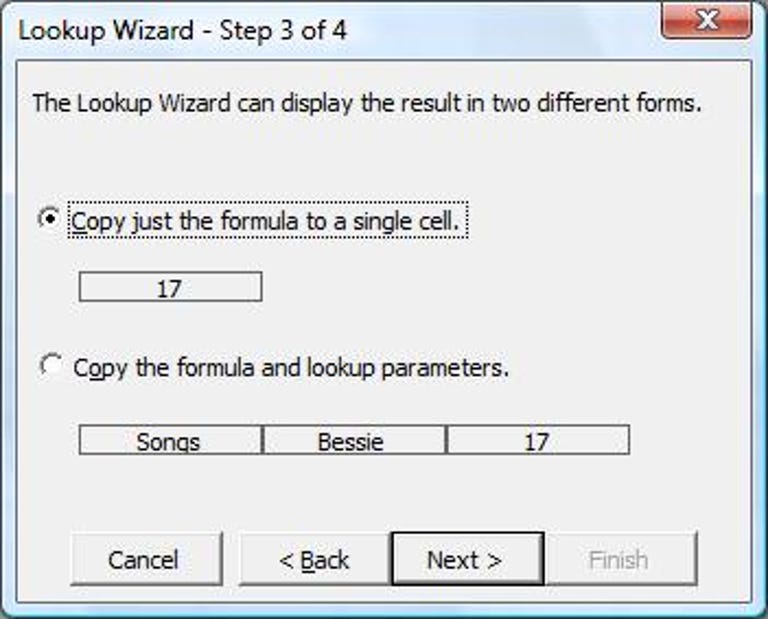
Choose the column containing the value you seek in the drop-down menu at the top of the wizard's second step, and note the value in the row field at the bottom of the dialog box, but don't change it. Click Next to move on to step 3. Choose Copy just the formula to a single cell, and click Next to open the fourth and last step of the wizard. Now click inside the empty text field of the last dialog box, then click the cell in the worksheet you want the data you're searching for to appear in, and choose Finish.
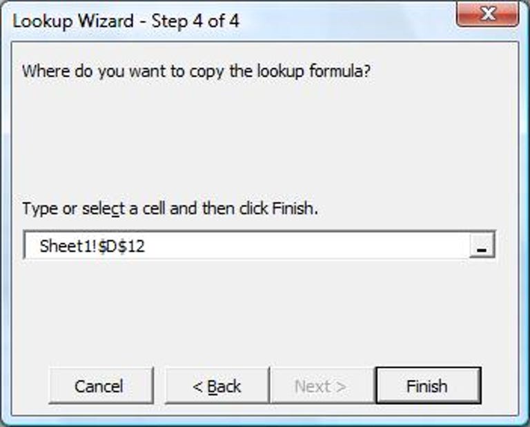
Back in your worksheet, select the cell containing the new formula, and change the formula value you noted in step 3 to the row containing the data you're looking for. To display the value of another row in that column, simply change the value again. In my music library example, I first searched for the value "Bessie" to show the number of songs recorded by Bessie Smith, and then I changed that value to "Emmylou" to display the number of songs in my library recorded by Emmylou Harris.
You now have a mini-worksheet search engine, but there's more you can do with the wizard, such as using it to find a range of cell values, or to display the values of two cells that are related in some way (by selecting the Copy the formula and lookup values option in step 3 of the wizard). I'll describe other lookup tricks in a future post.
Tomorrow: super productivity-enhancing Firefox extensions.