Five easy Excel formatting tricks

I've never trained an elephant, but I imagine the process is similar to that of getting your Microsoft Excel worksheet to look just right. Here are five of my favorite Excel formatting tricks.

Double-click to fit columns and rows
When you enter or paste text and numbers into Excel, the cells don't expand to fit their contents. The fast way to autofit columns and rows is to hover your mouse over the header border between the column and its neighbor to the right, or between two rows at the far left of the worksheet. When the resize icon appears, double-click.

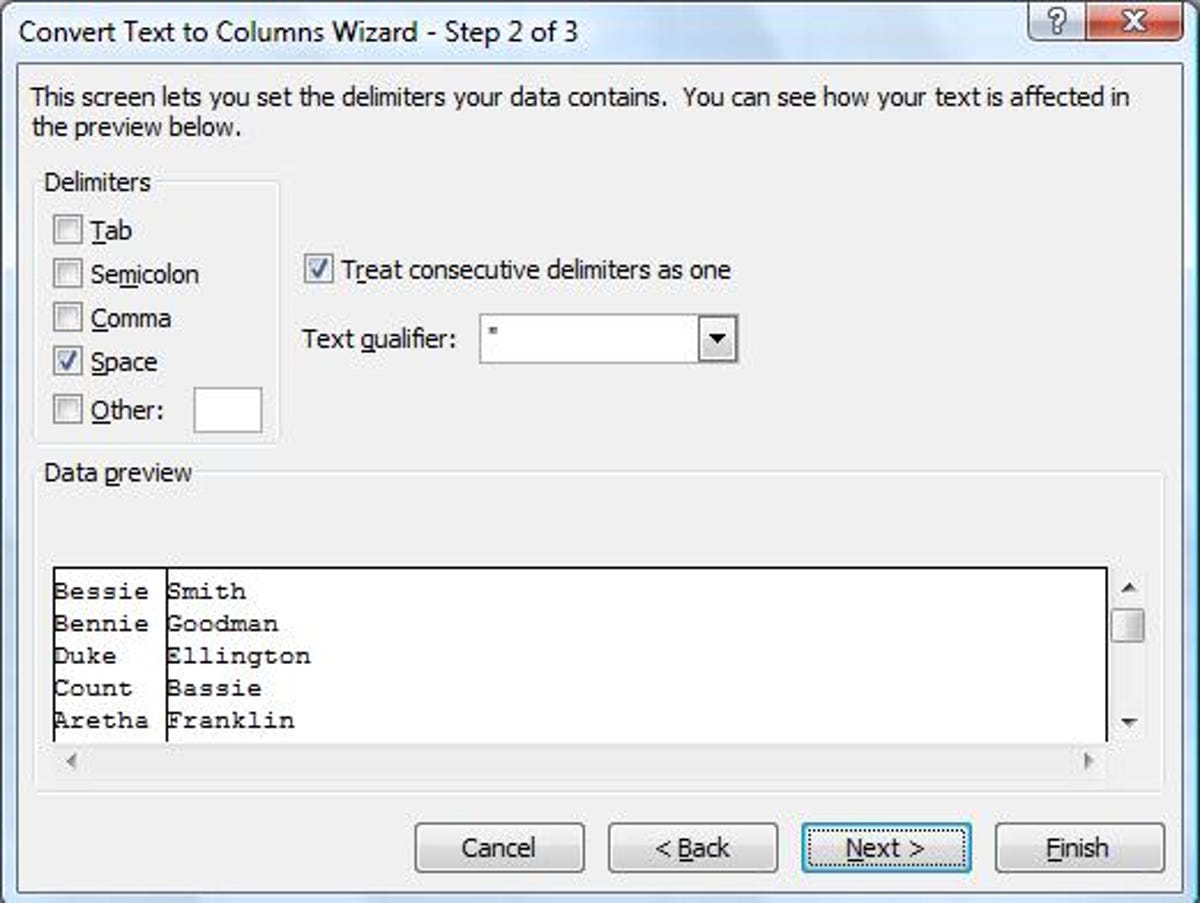
Convert one column into two
Suppose you have a list of full names in a column, and you'd like to separate the first names from the last names. In Excel 2003, select the column and click Data*Text to Columns. In Excel 2007, click the Data tab, and select the Text to Columns button. In both versions, choose Delimited (unless all the entries are the same length, in which case you can select Fixed width), click Next, and check Space (or whichever option applies; see the screen below). You can leave "Treat consecutive delimiters as one" checked. Click Next again to view data-formatting options, and then Finish.

At this point, you may want to change the order of the columns. To do so, simply select the column header, right-click the selection, and choose Cut. Now click the header of the blank column you want to place the cut cells in, right-click, and select Insert Cut Cells.

Paste formatting with one keystroke
If you'd like several disconnected cells to share a format, such as bold text and a background color, it can be a hassle to select each cell one at a time, open its cell-format dialog box, and make the changes you want. Instead, reformat one of the cells, and then select all of the others by pressing Ctrl, and clicking them one by one. Once they're all highlighted, press F4 to apply the formatting to all of them at once.

See your page breaks
I've been surprised so often when trying to print a worksheet that I automatically preview everything before I send it to the printer. You can get Excel to give you a visual cue about your page layouts by having it display page breaks. This option is the default in Excel 2007, but if your page breaks aren't showing, click the Office button, select Excel Options at the bottom of the window, choose Advanced in the left pane, scroll in the right to the display options, check Show page breaks, and click OK. Page breaks don't appear by default in Excel 2003 worksheets, so to show them, click Tools*Options*View, check Page breaks under Window options, and click OK.

Freeze your column headings
Scrolling through a big worksheet becomes a guessing game once you lose sight of the column headings. To keep them in view as you move down the rows in Excel 2003, select the row directly below the headings, and click Window*Freeze Panes. In Excel 2007, click the View tab, choose the Freeze Panes button, and select Freeze Top Row.

Monday: Get more out of your browser.