A scientific formula for popularity on Digg, YouTube

Get your own at Scribd or explore others: Technology Web 2.0 digg HP

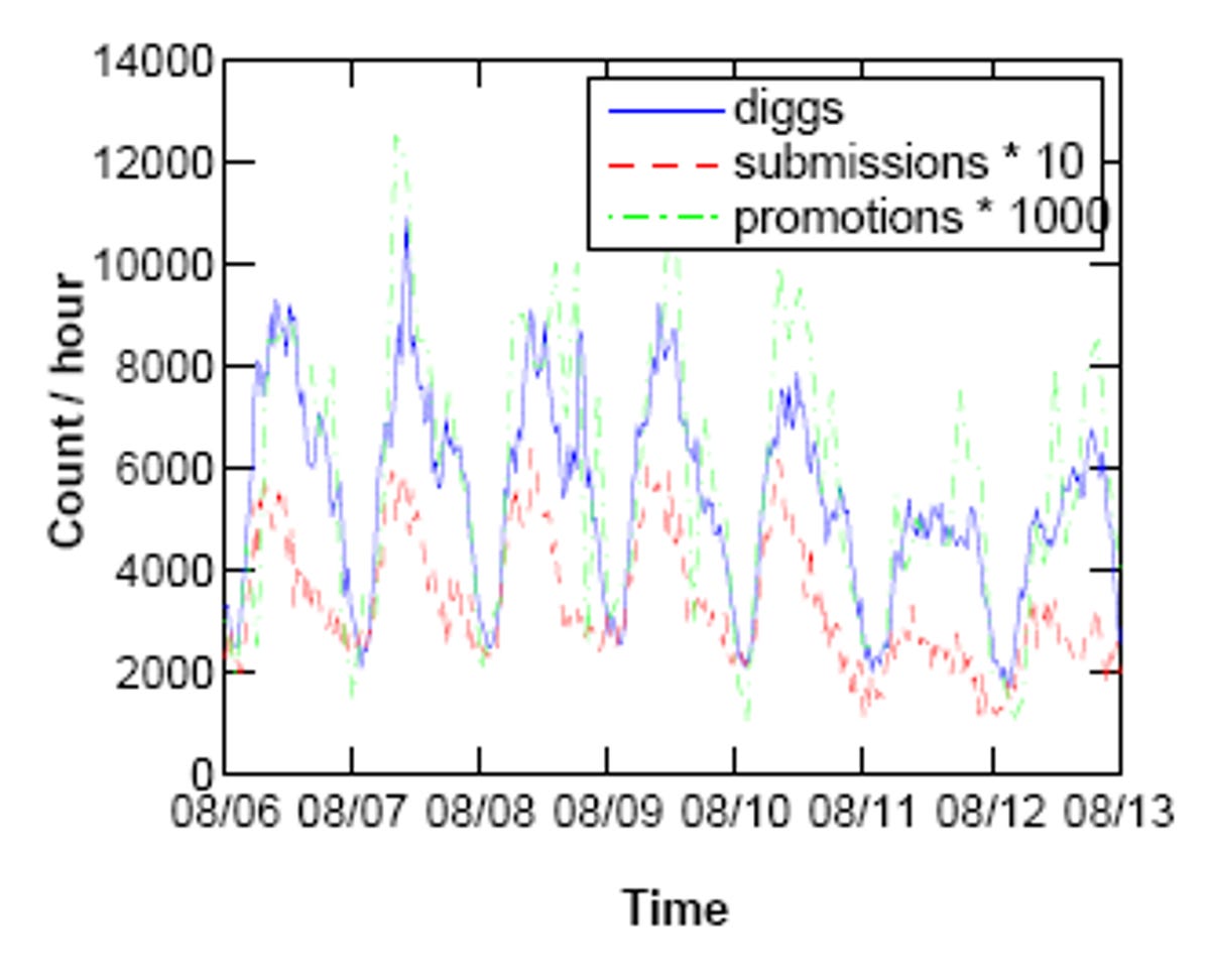
Predicting the popularity of online content Gabor Szabo Social Computing Lab HP Labs Palo Alto, CA Bernardo A. Huberman Social Computing Lab HP Labs Palo Alto, CA gabors@hp.com bernardo.huberman@hp.com ABSTRACT We present a method for accurately predicting the long time popularity of online content from early measurements of user's access. Using two content sharing portals, Youtube and Digg, we show that by modeling the accrual of views and votes on content offered by these services we can predict the long-term dynamics of individual submissions from initial data. In the case of Digg, measuring access to given stories during the first two hours allows us to forecast their popularity 30 days ahead with remarkable accuracy, while downloads of Youtube videos need to be followed for 10 days to attain the same performance. The differing time scales of the predictions are shown to be due to differences in how content is consumed on the two portals: Digg stories quickly become outdated, while Youtube videos are still found long after they are initially submitted to the portal. We show that predictions are more accurate for submissions for which attention decays quickly, whereas predictions for evergreen content will be prone to larger errors. The ease with which content can now be produced brings to the center the problem of the attention that can be devoted to it. Recently, it has been shown that attention [22] is allocated in a rather asymmetric way, with most content getting some views and downloads, whereas only a few receive the bulk of the attention. While it is possible to predict the distribution in attention over many items, so far it has been hard to predict the amount that would be devoted over time to given ones. This is the problem we solve in this paper. Most often portals rank and categorize content based on its quality and appeal to users. This is especially true of aggregators where the "wisdom of the crowd" is used to provide collaborative filtering facilities to select and order submissions that are favored by many. One such well-known portal is Digg, where users submit links and short descriptions to content that they have found on the Web, and others vote on them if they find the submission interesting. The articles collecting the most votes are then exhibited on premiere sections across the site, such as the "recently popular submissions" (the main page), and "most popular of the day/week/month/year". This results in a positive feedback mechanism that leads to a "rich get richer" type of vote accrual for the very popular items, although it is also clear that this pertains to only a very small fraction of the submissions. As a parallel to Digg, where content is not produced by the submitters themselves but only linked to it, we study Youtube, one of the first video sharing portals that lets users upload, describe, and tag their own videos. Viewers can watch, reply to, and leave comments on them. The extent of the online ecosystem that has developed around the videos on Youtube is impressive by any standards, and videos that draw a lot of viewers are prominently exposed on the site, similarly to Digg stories. The paper is organized as follows. In Section 2 we describe how we collected access data on submissions on Youtube and Digg. Section 3 shows how daily or weekly fluctuations can be observed in Digg, together with presenting a simple method to eliminate them for the sake of more accurate predictions. In Section 4 we discuss the models used to describe content popularity and how prediction accuracy depends on their choice. Here we will also point out that the expected growth in popularity of videos on Youtube is markedly different from when compared to Digg, and further study the reasons for this in Section 5. In Section 6 we conclude and cite relevant works to this study. Keywords Youtube, Digg, prediction, popularity, videos 1. INTRODUCTION The ubiquity and inexpensiveness of Web 2.0 services have transformed the landscape of how content is produced and consumed online. Thanks to the web, it is possible for content producers to reach out to audiences with sizes that are inconceivable using conventional channels. Examples of the services that have made this exchange between producers and consumers possible on a global scale include video, photo, and music sharing, weblogs and wikis, social bookmarking sites, collaborative portals, and news aggregators where content is submitted, perused, and often rated and discussed by the user community. At the same time, the dwindling cost of producing and sharing content has made the online publication space a highly competitive domain for authors. 2. SOURCES OF DATA The formulation of the prediction models relies heavily on observed characteristics of our experimental data, which we describe in this section. The organization of Youtube and Digg is conceptually similar to each other, so we can also employ a similar framework to study content popularity after the data has been normalized. To simplify the terminology, by popularity in the following we will refer to the number of views that a video receives on Youtube, and to the number of votes (diggs) that a story collects on Digg, respectively. 2.1 Youtube Youtube is the pinnacle of user-created video sharing portals on the Web, with 65,000 new videos uploaded and 100 million downloaded on a daily basis, implying that that 60% of all online videos are watched through the portal [11]. Youtube is also the third most frequently accessed site on the Internet based on traffic rank [11, 6, 3]. We started collecting view count time series on 7,146 selected videos daily, beginning April 21, 2008, on videos that appeared in the "recently added" section of the portal on this day. Apart from the list of most recently added videos, the web site also offers listings based on different selection criteria, such as "featured", "most discussed", and "most viewed" lists, among others. We chose the most recently uploaded list to have an unbiased sample of all videos submitted to the site in the sampling period, not only the most popular ones, and also so that we can have a complete history of the view counts for each video during their lifetime. The Youtube application programming interface [23] gives programmatic access to several of a video's statistics, the view count at a given time being one of them. However, due to the fact that the view count field of a video does not appear to be updated more often than once a day by Youtube, it is only possible to have a good approximation for the number of views daily. Within a day, however, the API does indicate when the view count was recorded. It is worth noting that while the overwhelming majority of video views is initiated from the Youtube website itself, videos may be linked from external sources as well (about half of all videos are thought to be linked externally, but also that only about 3% of the views are coming from these links [5]). In Section 4, we compare the view counts of videos at given times after their upload. Since in most cases we only have information on the view counts once a day, we use linear interpolation between the nearest measurement points around the time of interest to approximate the view count at the given time. as a massive collaborative filtering tool to select and show the most popular content, and thus registered users can digg submissions they found interesting. This serves to increase the digg count of the submission by one, and submissions that get substantially enough diggs in a relatively short time in the upcoming section will be presented on the front page of Digg, or using its terminology, they will be promoted to the front page. Someone's submission being promoted is a considerable source of pride in the Digg community, and is a main motivator for returning submitters. The exact algorithm for promotion is not made public to thwart gaming, but is thought to give preference to upcoming submissions that accumulate diggs quickly enough from diverse neighborhoods of the Digg social network [18]. The social networking feature offered by Digg is extremely important, through which users may place watch lists on another user by becoming their "fans". Fans will be shown updates on which submissions users dugg who they are fans of, and thus the social network will play a major role in making upcoming submissions more visible. Very importantly, in this paper we also only consider stories that were promoted to the front page, given that we are interested in submissions' popularity among the general user base rather than in niche social networks. We used the Digg API [8] to retrieve all the diggs made by registered users between July 1, 2007, and December 18, 2007. This data set comprises of about 60 million diggs by 850 thousand users in total, cast on approximately 2.7 million submissions (this number includes all past submissions also that received any digg). The number of submissions in this period was 1,321,903, of which 94,005 (7.1%) became promoted to the front page. 3. DAILY CYCLES In this section we examine the daily and weekly activity variations in user activity. Figure 1 shows the hourly rates of digging and story submitting of users, and of upcoming story promotions by Digg, as a function of time for one week, starting August 6, 2007. The difference in the rates may be as much as threefold, and weekends also show lesser activity. Similarly, Fig. 1 also showcases weekly variations, where weekdays appear about 50% more active than weekends. It is also reasonable to assume that besides daily and weekly cycles, there are seasonal variations as well. It may also be concluded that Digg users are mostly located in the UTC-5 to UTC-8 time zones, and since the official language of Digg is English, Digg users are mostly from North America. Depending on the time of day when a submission is made to the portal, stories will differ greatly on the number of initial diggs that they get, as Fig. 2 illustrates. As can be expected, stories submitted at less active periods of the day will accrue less diggs in the first few hours initially than stories submitted during peak times. This is a natural consequence of suppressed digging activity during the nightly hours, but may initially penalize interesting stories that will ultimately become popular. In other words, based on observations made only after a few hours after a story has been promoted, we may misinterpret a story's relative interestingness, if we do not correct for the variation in daily activity cycles. For instance, a story that gets promoted at 12pm will on average get approximately 400 diggs in the first 2 2.2 Digg Digg is a Web 2.0 service where registered users can submit links and short descriptions to news, images, or videos they have found interesting on the Web, and which they think should hold interest for the greater general audience, too (90.5% of all uploads were links to news, 9.2% to videos, and only 0.3% to images). Submitted content will be placed on the site in a so-called "upcoming" section, which is one click away from the main page of the site. Links to content are provided together with surrogates for the submission (a short description in the case of news, and a thumbnail image for images and videos), which is intended to entice readers to peruse the content. The main purpose of Digg is to act 14000 12000 Average number of diggs diggs submissions * 10 promotions * 1000 1000 800 600 400 200 0 0 Count / hour 10000 8000 6000 4000 2000 0 08/06 08/07 08/08 08/09 08/10 08/11 08/12 08/13 5 10 15 20 25 Time Promotion hour of day Figure 1: Daily and weekly cycles in the hourly rates of digging activity, story submissions, and story promotions, respectively. To match the different scales the rates for submissions is multiplied by 10, that of the promotions is multiplied by 1000. The horizontal axis represents one week from August 6, 2007 (Monday) through Aug 12, 2007 (Sunday). The tick marks represent midnight of the respective day, Pacific Standard Time. hours, while it will only get 200 diggs if it is promoted at midnight. Since the digging activity varies by time, we introduce the notion of digg time, where we measure time not by wall time (seconds), but by the number of all diggs that users cast on promoted stories. We choose to count diggs only on promoted stories only because this is the section of the portal that we focus on stories from, and most diggs (72%) are going to promoted stories anyway. The average number of diggs arriving to promoted stories per hour is 5,478 when calculated over the full data collection period, thus we define one digg hour as the time it takes for so many new diggs to be cast. As seen earlier, during the night this will take about three times longer than during the active daily periods. This transformation allows us to mitigate the dependence of submission popularity on the time of day when it was submitted. When we refer to the age of a submission in digg hours at a given time t, we measure how many diggs were received in the system between t and the submission of the story, and divide by 5,478. A further reason to use digg time instead of absolute time will be given in Section 4.1. Figure 2: The average number of diggs that stories get after a certain time, shown as a function of the hour that the story was promoted at (PST). Curves from bottom to top correspond to measurements made 2, 4, 8, and 24 hours after promotion, respectively. with respect to the upload (promotion) time is tr . By indicator time ti we refer to when in the life cycle of the submission we perform the prediction, or in other words how long we can observe the submission history in order to extrapolate; ti < tr . 4.1 Correlations between early and later times We first consider the question whether the popularity of submissions early on is any predictor of their popularity at a later stage, and if so, what the relationship is. For this, we first plot the popularity counts for submissions at the reference time tr = 30 days both for Digg (Fig. 3) and Youtube (Fig. 4), versus the popularities measured at the indicator times ti = 1 digg hour, and ti = 7 days for the two portals, respectively. We choose to measure the popularity of Youtube videos at the end of the 7th day so that the view counts at this time are in the 101 -104 range, and similarly for Digg in this measurement. We logarithmically rescale the horizontal and vertical axes in the figures due to the large variances present among the popularities of different submissions (notice that they span three decades). Observing the Digg data, one notices that the popularity of about 11% of stories (indicated by lighter color in Fig. 3) grows much slower than that of the majority of submissions: by the end of the first hour of their lifetime, they have received most of the diggs that they will ever get. The separation of the two clusters is perceivable until approximately the 7th digg hour, after which the separation vanishes due to fact that by that time the digg counts of stories mostly saturate to their respective maximum values (skip to Fig. 10 for the average growth of Digg article popularities). While there is no obvious reason for the presence of clustering, we assume that it arises when the promotion algorithm of Digg misjudges the expected future popularity of stories, and promotes stories from the upcoming phase that will not maintain a sustained attention from the users. Users thus lose 4. PREDICTIONS In this section we show that if we perform a logarithmic transformation on the popularities of submissions, the transformed variables exhibit strong correlations between early and later times, and on this scale the random fluctuations can be expressed as an additive noise term. We use this fact to model and predict the future popularity of individual content, and measure the performance of the predictions. In the following, we call reference time tr the time when we intend to predict the popularity of a submission whose age 10 4 Popularity after 30 digg days Popularity after 30 days 10 10 10 10 10 5 4 10 3 3 2 10 2 1 10 1 10 1 10 2 10 3 10 0 10 0 10 1 10 2 10 3 10 4 10 5 Popularity after 1 digg hour Popularity after 7 days Figure 3: The correlation between digg counts on the 17,097 promoted stories in the dataset that are older than 30 days. A k-means clustering separates 89% of the stories into the upper cluster, while the rest of the stories is shown in lighter color. The bold guide line indicates a linear fit with slope 1 on the upper cluster, with a prefactor of 5.92 (the Pearson correlation coefficient is 0.90). The dashed line marks the y = x line below which no stories can fall. Figure 4: The popularities of videos shown at the 30th day after upload, versus their popularity after 7 days. The bold solid line with gradient 1 has been fit to the data, with correlation coefficient R = 0.77 and prefactor 2.13. this is the time scale of the strongest daily variations (cf. Fig. 1). We do not show the untransformed scale PCC for Digg submissions measured in digg hours, since it approximately traces the dashed line in the figure, thus also indicating a weaker correlation than the solid line. interest in them much sooner than in stories in the upper cluster. We used k-means clustering with k = 2 and cosine distance measure to separate the two clusters as shown in Fig. 3 up to the 7th digg hour (after which the clusters are not separable), and we exclusively use the upper cluster for the calculations in the following. As a second step, to quantify the strength of the correlations apparent in Figs. 3 and 4, we measured the Pearson correlation coefficients between the popularities at different indicator times and the reference time. The reference time is always chosen tr = 30 days (or digg days for Digg) as previously, and the indicator time is varied between 0 and tr . Youtube. Fig. 5 shows the Pearson correlation coefficients between the logarithmically transformed popularities, and for comparison also the correlations between the untransformed variables. The PCC is 0.92 after about 5 days; however, the untransformed scale shows weaker linear dependence, at 5 days the PCC is only 0.7, and it consistently stays below the PCC of the logarithmically transformed scale. Digg. Also in Fig. 5, we plot the PCCs of the log-transformed popularities between the indicator times and the reference time. It is already 0.98 after the 5th digg hour, and it is as strong as 0.993 after the 12th. We also argue here that by measuring submission age as digg time leads to stronger correlations: the figure shows the PCC as well for the case when the story age is measured as absolute time (dashed line, 17,222 stories), and it is always less than the PCCs taken with digg hours (solid line, 17,097 stories) up to approximately the 12th hour. This is understandable since 4.2 The evolution of submission popularity The strong linear correlation found between the indicator and reference times of the logarithmically transformed submission popularities suggests that the more popular submissions are in the beginning, the more they will be also later on, and the connection can be described by a linear model: ln Ns (t2 ) = = ln [r(t1 , t2 )Ns (t1 )] + ξs (t1 , t2 ) ln r(t1 , t2 ) + ln Ns (t1 ) + ξs (t1 , t2 ), (1) where Ns (t) is the popularity of submission s at time t (in the case of Digg, time is naturally measured by digg time), and t1 and t2 are two arbitrarily chosen points in time, t2 > t1 . r(t1 , t2 ) accounts for the linear relationship found between the log-transformed popularities at different times, and it is independent of s. ξs is a noise term drawn from a given distribution with mean 0 that describes the randomness observed in the data. It is important to note that the noise term is additive on the log-scale of popularities, justified by the fact that the strongest correlations were found on this transformed scale. Considering Figures 3 and 4, the popularities at t2 = tr also appear to be evenly distributed around the linear fit (with taking only the upper cluster in Fig. 3 and considering the natural cutoff y = x in Fig. 4). We will now show that the variations of the log-popularities around the expected average are distributed approximately normally with an additive noise. To this end we performed linear regression on the logarithmicalyy transformed data points shown in Figs. 3 and 4, respectively, fixing the slope of the linear regression function to 1 in accordance with Eq. (1). The intercept of the linear fit corresponds to ln r(ti , tr ) above (ti = 7 days/1 digg hour, tr = 30 days), and ξs (ti , tr ) are Pearson correlation coefficient 1 0.95 0.9 0.85 0.8 0.75 0.7 0 2 1200 1.5 1000 Residual quantiles Frequency 800 600 400 200 1 0.5 0 −0.5 −1 −1.5 −4 0 −1 −0.5 0 0.5 1 1.5 2 Residuals Youtube (days) Youtube (untr.) Digg (digg hours) Digg (hours) 5 10 15 −2 0 2 4 Time (days/hours/digg hours) Standard normal quantiles Figure 5: The Pearson correlation coefficients between the logarithms of the popularities of submissions measured at different times: at the time indicated by the horizontal axis, and on the 30th day. For Youtube, the x-axis is in days. For Digg, it is in hours for the dashed line, and digg hours for the solid line (stronger correlation). For comparison, the dotted line shows the correlation coefficients for the untransformed (non-logarithmic) popularities in Youtube. Figure 6: The quantile-quantile plot of the residuals of the linear fit of Fig. 3 to the logarithms of Digg story popularities, as described in the text. The inset shows the frequency distribution of the residuals. A further justification for the model of Eq. (1) is given in the following. It has been shown that the popularity distribution of Digg stories of a given age follows a lognormal distribution [22] that is the result of a growth mechanism with multiplicative noise, and can be described as ln Ns (t2 ) = ln Ns (t1 ) + t2 X given by the residuals of the variables with respect to the best fit. We tested the normality of the residuals by plotting the quantiles of their empirical distributions versus the quantiles of the theoretical (normal) distributions in Figs. 6 (Digg) and 7 (Youtube). The residuals show a reasonable match with normal distributions, although we observe in the quantilequantile plots that the measured distributions of the residuals are slightly right-skewed, which means that content with very high popularity values is overrepresented in comparison to less popular content. This is understandable if we consider that a small fraction of the submissions ends up on "most popular" and "top" pages of both portals. These are the submissions that are deemed most requested by the portals, and are shown to the users as those that others found most interesting. They stay on frequented and very visible parts of the portals, and are naturally attract further diggs/views. In the case of Youtube, one can see that content popularity at the 30th day versus the 7th day as shown in Fig. 4 is bounded from below, due to the fact the view counts can only grow, and thus the distribution of residuals is also truncated in Fig. 7. We also note that the Jarque-Bera and Lilliefors tests reject residual normality at the 5% significance level for both systems, although the residuals appear to be distributed reasonably close to Gaussians. Moreover, to see whether the homoscedasticity of the residuals holds that is necessary for the linear regression [their variance being independent of Ns (ti )], we checked the means and variances of the residuals as a function of Nc (ti ) by subdividing the popularity values into 50 bins, with the result that both the mean and variance are independent of Nc (ti ). η(τ ), (2) τ =t1 where η(*) denotes independent values drawn from a fixed probability distribution, and time is measured in discrete steps. If the difference between t1 and t2 is large enough, the distribution of the sum of η(τ )'s will approximate a normal distribution, according to the central limit theorem. We can thus map the mean of the sum of η(τ )'s to ln r(t1 , t2 ) in Eq. (1), and find that the two descriptions are equivalent characterizations of the same lognormal growth process. 4.3 Prediction models We present three models to predict an individual submission's popularity at a future time tr . The performance of the predictions is measured on the test sets by defining error functions that yield a measure of deviation of the predictions from the observed popularities at tr , and together with the models we discuss what error measure they are expected to minimize. One model that minimizes a given error function may fare worse for another error measure. The first prediction model closely parallels the experimental observations shown in the previous section. In the second, we consider a common error measure and formulate the model so that it is optimal with respect to this error function. Lastly, the third prediction method is presented as comparison and one that has been used in previous works as an "intuitive" way of modeling popularity growth [15]. Below, we use the x notation to refer to the predicted value ? of x at tr . 5 700 4 600 500 Residual quantiles 3 2 1 0 −1 −2 −4 400 300 200 100 0 −1 0 1 2 3 4 5 2 Here σ0 = var(rc ), the consistent estimate for the variance of the residuals on the logarithmic scale. Thus the procedure to estimate the expected popularity of a given submission s at time tr from measurements at time ti , we first determine the regression coefficient β0 (ti ) and the variance of the residuals 2 σ0 from the training set, and apply Eq. (5) to obtain the expectation on the original scale, using the popularity Ns (ti ) measured for s at ti . Frequency Residuals 4.3.2 CS model: constant scaling model; relative squared error −2 0 2 4 In this section we first define the error function that we wish to minimize, and then present a linear estimator for the predictions. The relative squared error that we use here takes the form of " #2 " #2 X Nc (ti , tr ) − Nc (tr ) X Nc (ti , tr ) ? ? RSE = = −1 . Nc (tr ) Nc (tr ) c c (6) This is similar to the commonly used relative standard error ˛ ˛ ˛? ˛ ˛ Nc (ti , tr ) − Nc (tr ) ˛ (7) ˛ ˛, ˛ ˛ Nc (tr ) except that the absolute value of the relative difference is replaced by a square. The linear correspondence found between the logarithms of the popularities up to a normally distributed noise term sug? gests that the future expected value Ns (ti , tr ) for submission s can be expressed as ? Ns (ti , tr ) = α(ti , tr )Ns (ti ). (8) Standard normal quantiles Figure 7: The quantile-quantile plot of the residuals of the linear fit of Fig. 4 for Youtube. 4.3.1 LN model: linear regression on a logarithmic scale; least-squares absolute error The linear relationship found for the logarithmically transformed popularities and described by Eq. (1) above suggests that given the popularity of a submission at a given time, a good estimate we can give for a later time is determined by the ordinary least squares estimate, and it is the best estimate that minimizes the sum of the squared residuals (a consequence of the linear regression with the maximum likelihood method). However, the linear regression assumes normally distributed residuals and the lognormal model gives rise to additive Gaussian noise only if the logarithms of the popularities are considered, and thus the overall error that is minimized by the linear regression on this scale is i2 X 2 Xh ? LSE∗ = rc = lnNc (ti , tr ) − ln Nc (tr ) , (3) c c ? where lnNc (ti , tr ) is the prediction for ln Nc (tr ), and is cal? culated as lnNc (ti , tr ) = β0 (ti ) + ln Nc (ti ) and β0 is yielded by the maximum likelihood parameter estimator for the intercept of the linear regression with slope 1. The sum in Eq. (3) goes over all content in the training set when estimating the parameters, and the test set when estimating the error. We, on the other hand, are in practice interested in the error on the linear scale, i2 Xh ? (4) Nc (ti , tr ) − Nc (tr ) . LSE = c α(ti , tr ) is independent of the particular submission s, and only depends on the indicator and reference times. The value that α(ti , tr ) takes, however, will be contingent on what the error function is, so that the optimal value of α minimizes this. We will minimize RSE on the training set if and only if - X » Nc (ti ) ∂RSE Nc (ti ) 0= =2 α(ti , tr ) − 1 . (9) ∂α(ti , tr ) Nc (tr ) Nc (tr ) c Expressing α(ti , tr ) from above, P c Nc (ti ) c N (t ) Nc (tr ) The residuals, while distributed normally on the logarithmic scale, will not have this property on the untransformed scale, and an inconsistent estimate would result if we used h i ? exp lnNc (ti , tr ) as a predictor on the natural (original) scale of popularities [9]. However, fitting least squares regression models to transformed data has been extensively investigated (see Refs. [9, 16, 21]), and in case the transformation of the dependent variable is logarithmic, the best untransformed scale estimate is ? ? 2 ? Ns (ti , tr ) = exp ln Ns (ti ) + β0 (ti ) + σ0 /2 . (5) The value of α(ti , tr ) can be calculated from the training data for any ti , and further, the prediction for any new submission may be made knowing its age using this value from the training set, together with Eq. (8). If we verified the error on the training set itself, it is guaranteed that RSE is minimized under the model assumptions of linear scaling. α(ti , tr ) = P h c r i2 . Nc (ti ) (10) 4.3.3 GP model: growth profile model For comparison, we consider a third description for predicting future content popularity, which is based on average growth profiles devised from the training set [15]. This assumes in essence that the growth of a submission's popularity in time follows a uniform accrual curve, which is appro- Digg Youtube Training set 10825 stories (7/1/07-9/18/07) 3573 videos randomly selected Test set 6272 stories (9/18/07-12/6/07) 3573 videos randomly selected prediction error measures for one particular submission s: h i2 ? (13) QSE(s, ti , tr ) = Ns (ti , tr ) − Ns (tr ) and QRE(s, ti , tr ) = " ? Ns (ti , tr ) − Ns (tr ) Ns (tr ) #2 . (14) Table 1: The partitioning of the collected data into training and test sets. The Digg data is divided by time while the Youtube videos are chosen randomly for each set, respectively. priately rescaled to account for the differences between submission interestingnesses. The growth profile is calculated on the training set as the average of the relative popularities of the submissions of a given age ti , as normalized by the final popularity at the reference, tr : fi fl Nc (t0 ) P (t0 , t1 ) = , (11) Nc (t1 ) c where * c takes the mean of its argument over all content in the training set. We assume that the rescaled growth profile approximates the observed popularities well over the whole time axis with an affine transformation, and thus at ti the rescaling factor Πs is given by Ns (ti ) = Πs (ti , tr )P (ti , tr ). The prediction for tr consists of using Πs (ti , tr ) to calculate the future popularity, Ns (ti ) ? Ns (tr ) = Πs (ti , tr )P (tr , tr ) = Πs (ti , tr ) = . (12) P (ti , tr ) The growth profiles for Youtube and Digg were measured and shown in Fig. 10. QSE(s, ti , tr ) is the squared difference between the prediction and the actual popularity for a particular submission s, and QRE is the relative squared error. We will use this notation to refer to their ensemble average values, too, QSE = QSE(c, ti , tr ) c , where c goes over all submissions in the test set, and similarly, QRE = QRE(s, ti , tr ) c . We used the parameters obtained in the learning session to perform the predictions on the test set, and plotted the resulting average error values calculated with the above error measures. Figure 8 shows QSE and QRE as a function of ti , together with their respective standard deviations. ti , as earlier, is measured from the time a video is presented in the recent list or when a story gets promoted to the front page of Digg. QSE, the squared error is indeed smallest for the LN model for Digg stories in the beginning, then the difference between the three models becomes modest. This is expected since the LN model optimizes for the RSE objective function, which is equivalent to QSE up to a constant factor. Youtube videos do not show remarkable differences against any of the three models, however. A further difference between Digg and Youtube is that QSE shows considerable dispersion for Youtube videos over the whole time axis, as can be seen from the large values of the standard deviation (the shaded areas in Fig. 8). This is understandable, however, if we consider that the popularity of Digg news saturates much earlier than that of Youtube videos, as will be studied in more detail in the following section. Considering further Fig. 8 (b) and (d), we can observe that the relative expected error QRE decreases very rapidly for Digg (after 12 hours it is already negligible), while the predictions converge slower to the actual value in the case of Youtube. Here, however, the CS model outperforms the other two for both portals, again as a consequence of finetuning the model to minimize the objective function RSE. It is also apparent that the variation of the prediction error among submissions is much smaller than in the case of QSE, and the standard deviation of QRE is approximately proportional to QRE itself. The explanation for this is that the noise fluctuations around the expected average as described by Eq. (1) are additive on a logarithmic scale, which means that taking the ratio of a predicted and an actual popularity as in QRE is translated into a difference on the logarithmic scale of popularities. The difference of the logs is commensurate with the noise term in Eq. (1), thus stays bounded in QRE, and is instead amplified multiplicatively in QSE. In conclusion, for relative error measures the CS model should be chosen, while for absolute measures the LN model is a good choice. 4.4 Prediction performance The performance of the prediction methods will be assessed in this section, using two error functions that are analogous to LSE and RSE, respectively. We subdivided the submission time series data into a training set and a test set, on which we benchmarked the different prediction schemes. For Digg, we took all stories that were submitted during the first half of the data collection period as the training set, and the second half was considered as the test set. On the other hand, the 7,146 Youtube videos that we followed were submitted around the same time, so instead we randomly selected 50% of these videos as training and the other half as test. The number of submissions that the training and test sets contain are summarized in Table 1. The parameters defined in the prediction models were found 2 through linear regression (β0 and σ0 ) and sample averaging (α and P ), respectively. For reference time tr where we intend to predict the popularity of submissions we chose 30 days after the submission time. Since the predictions naturally depend on ti and how close we are to the reference time, we performed the parameter estimations in hourly intervals starting after the introduction of any submission. Analogously to LSE and RSE, we will consider the following 5. SATURATION OF THE POPULARITY 1000 Relative squared error 800 LN CS GP 0.5 0.4 0.3 0.2 0.1 0 0 LN CS GP Squared error 600 400 200 0 0 0.5 1 1.5 2 0.2 0.4 0.6 0.8 1 (a) 8000 Digg story age (digg days) (b) 1 Digg story age (digg days) Relative squared error Squared error 6000 LN CS GP 0.8 0.6 0.4 0.2 0 0 LN CS GP 4000 2000 0 0 5 10 15 20 25 30 5 10 15 20 25 30 (c) Youtube video age (days) (d) Youtube video age (days) Figure 8: The performance of the different prediction models, measured by two error functions as defined in the text: the absolute squared error QSE [(a) and (c)], and the relative squared error QRE [(b) and (d)], respectively. (a) and (b) show the results for Digg, while (c) and (d) for Youtube. The shaded areas indicate one standard deviation of the individual submission errors around the average. Average normalized popularity 1 Relative squared error 0.8 0.6 0.4 0.2 0 0 Digg Youtube 1.2 1 0.8 1 Digg Youtube 0.6 0.4 0.2 0 0 5 10 15 0.8 0.6 0.4 0.2 0 0 10 20 30 40 Time (digg hours) 20 40 60 80 100 20 25 30 Percentage of final popularity Time (days) Figure 9: The relative squared error shown as a function of the percentage of the final popularity of submissions on day 30. The standard deviations of the errors are indicated by the shaded areas. Figure 10: Average normalized popularities of submissions for Youtube and Digg by the popularity at day 30. The inset shows the same for the first 48 digg hours of Digg submissions. Here we discuss how the trends in the growth of popularities in time are different for Youtube and Digg, and how this generally affects the predictions. As seen in the previous section, the predictions converge much faster for Digg articles than for videos on Youtube to their respective reference values, and the explanation can be found when we consider how the popularity of submissions approaches the reference values. In Fig. 9 we show an analogous interpretation of QRE, but instead of plotting the error against time, we plotted it as a function of the actual popularity, expressed as the fraction of reference value Ns (tr ). The plots are averages over all content in the test set, and over times ti in hourly increments up to tr . This means that the predictions across Youtube and Digg become comparable, since we can eliminate the effect of the different time dynamics imposed on content popularity by the visitors that are idiosyncratic to the two different portals: the popularity of Digg submissions initially grows much faster, but it quickly saturates to a constant value, while Youtube videos keep getting views constantly (Fig. 10). As Fig. 9 shows, the average error QRE for Digg articles converges to 0 as we approach the reference time, with variations in the error staying relatively small. On the other hand, the same error measure does not decrease monotonically for Youtube videos until very close to the reference, which means that the growth of popularity of videos still shows considerable fluctuations near the 30st day, too, when the popularity is already almost as large as the reference value. This fact is further illustrated by Fig. 10, where we show the average normalized popularities for all submissions. This is calculated by dividing the popularity counts of individual submission by their reference popularities on day 30, and averaging the resulting normalized functions over all content. An important difference that is apparent in the figure is that while Digg stories saturate fairly quickly (in about one day) to their respective reference popularities, Youtube videos keep getting views all throughout their lifetime (at least throughout the data collection period, but it is expected that the trendline continues almost linearly). The rate at which videos keep getting views may naturally differ among videos: less popular videos in the beginning are likely to show a slow pace over longer time scales, too. It is thus not surprising that the fluctuations around the average are not getting supressed for videos as they age (compare with Fig. 9). We also note that the normalized growth curves shown in Fig. 10 are exactly P (ti , tr ) of Eq. (11) when tr = 30 days. The mechanism that gives rise to these two markedly different behaviors is a consequence of the different ways of how users find content on the two portals: on Digg, articles become obsolete fairly quickly, since they oftenmost refer to breaking news, fleeting Internet fads, or technology-related stories that naturally have a limited time period while they interest people. Videos on Youtube, however, are mostly found through search, since due to the sheer amount of videos uploaded constantly it is not possible to match Digg's way of giving exposure to each promoted story on a front page (except for featured videos, but here we did not consider those separately). The faster initial rise of the popularity of videos can be explained by their exposure on the "recently added" tab of Youtube, but after they leave that section of the site, the only way to find them is through keyword search or when they are displayed as related videos with another video that is being watched. It serves thus an explanation to why the predictions converge faster for Digg stories than Youtube videos (10% accuracy is reached within about 2 hours on Digg vs. 10 days on Youtube) that the popularities of Digg submissions do not change considerably after 2 days. 6. CONCLUSIONS AND RELATED WORK In this paper we presented a method and experimental verification on how the popularity of (user contributed) content can be predicted very soon after the submission has been made, by measuring the popularity at an early time. A strong linear correlation was found between the logarithmically transformed popularities at early and later times, with the residual noise on this transformed scale being normally distributed. Using the fact of linear correlation we presented three models for making predictions about future popularity, and compared their performance on Youtube videos and Digg story submissions. The multiplicative nature of the noise term allows us to show that the accuracy of the predictions will exhibit a large dispersion around the average if a direct squared error measure is chosen, while if we take the relative errors the dispersion is considerably smaller. An important consequence is that absolute error measures should be avoided in favor of relative measures in community portals when the error of the prediction is estimated. We mention two scenarios where predictions of individual content can be used: advertising and content ranking. If the popularity count is tied to advertising revenue such as what results from advertisement impressions shown beside a video, the revenue may be fairly accurately estimated, since the uncertainty of the relative errors stays acceptable. However, when the popularities of different content are compared to each other as commonly done in ranking and presenting the most popular content to users, it is expected that the precise forecast of the ordering of the top items will be more difficult due to the large dispersion of the popularity count errors. We based the predictions of future popularities only on values measurable in the present, but did not consider the semantics of popularity and why some submissions become more popular than others. We believe that in the presence of a large user base predictions can essentially be made on observed early time series, and semantic analysis of content is more useful when no early clickthrough information is known for content. Furthermore, we argue for the generality of performing maximum likelihood estimates for the model parameters in light of a large amount of experimental information, since in this case Bayesian inference and maximum likelihood methods essentially yield the same estimates [14]. There are several areas that we could not explore here. It would be interesting to extend the analysis by focusing on different sections of the Web 2.0 portals, such as how the "news & politics" category differs from the "entertainment" section on Youtube, since we expect that news videos reach obsolescence sooner than videos that are recurringly searched for for a long time. It is also to be seen if it is possi- ble to forecast a Digg submission's popularity when the diggs are coming from a small number of users only whose voting history is known, as is the case for stories in the upcoming section of Digg. In related works video on demand systems and properties of media files on the Web have been studied in detail, statistically characterizing video content in terms of length, rank, and comments [6, 1, 19]. Video characteristics and user access frequencies are studied together when streaming media workload is estimated [11, 7, 13, 24]. User participation and content rating is also modeled in Digg, with particular emphasis on the social network and the upcoming phase of stories [18]. Activity fluctuations, user commenting behavior prediction, the ensuing social network, and community moderation structure is the focus of studies on Slashdot [15, 12, 17], a portal that is similar in spirit to Digg. The prediction of user clickthrough rates as a function of document and search engine result ranking order has overlaps with this paper [4, 2]. While the display ordering of submissions plays a less important role for the predictions presented here, Dupret et al. studied the effect of document position in a list on its selection probability with a Bayesian network model that becomes important when static content is predicted [10]; a related area is online ad clickthrough rate prediction also [20]. [10] [11] [12] [13] [14] [15] 7. REFERENCES [16] [1] S. Acharya, B. Smith, and P. Parnes. Characterizing User Access To Videos On The World Wide Web. In Proc. SPIE, 2000. [2] E. Agichtein, E. Brill, S. Dumais, and R. Ragno. Learning user interaction models for predicting web search result preferences. In SIGIR '06: Proceedings of the 29th annual international ACM SIGIR conference on Research and development in information retrieval, pages 3-10, New York, NY, USA, 2006. ACM. [3] Alexa Web Information Service, http://www.alexa.com. [4] K. Ali and M. Scarr. Robust methodologies for modeling web click distributions. In WWW '07: Proceedings of the 16th international conference on World Wide Web, pages 511-520, New York, NY, USA, 2007. ACM. [5] M. Cha, H. Kwak, P. Rodriguez, Y.-Y. Ahn, and S. Moon. I tube, you tube, everybody tubes: analyzing the world's largest user generated content video system. In IMC '07: Proceedings of the 7th ACM SIGCOMM conference on Internet measurement, pages 1-14, New York, NY, USA, 2007. ACM. [6] X. Cheng, C. Dale, and J. Liu. Understanding the characteristics of internet short video sharing: Youtube as a case study, 2007, arxiv:0707.3670v1. [7] M. Chesire, A. Wolman, G. M. Voelker, and H. M. Levy. Measurement and analysis of a streaming-media workload. In USITS'01: Proceedings of the 3rd conference on USENIX Symposium on Internet Technologies and Systems, pages 1-1, Berkeley, CA, USA, 2001. USENIX Association. [8] Digg application programming interface, http://apidoc.digg.com/. [9] N. Duan. Smearing estimate: A nonparametric [17] [18] [19] [20] [21] [22] [23] [24] retransformation method. Journal of the American Statistical Association, 78(383):605-610, 1983. G. Dupret, B. Piwowarski, C. A. Hurtado, and M. Mendoza. A statistical model of query log generation. In SPIRE, pages 217-228, 2006. P. Gill, M. Arlitt, Z. Li, and A. Mahanti. Youtube traffic characterization: a view from the edge. In IMC '07: Proceedings of the 7th ACM SIGCOMM conference on Internet measurement, pages 15-28, New York, NY, USA, 2007. ACM. V. G´mez, A. Kaltenbrunner, and V. L´pez. o o Statistical analysis of the social network and discussion threads in slashdot. In WWW '08: Proceeding of the 17th international conference on World Wide Web, pages 645-654, New York, NY, USA, 2008. ACM. M. J. Halvey and M. T. Keane. Exploring social dynamics in online media sharing. In WWW '07: Proceedings of the 16th international conference on World Wide Web, pages 1273-1274, New York, NY, USA, 2007. ACM. J. Higgins. Bayesian inference and the optimality of maximum likelihood estimation. International Statistical Review, 45:9-11, 1977. A. Kaltenbrunner, V. Gomez, and V. Lopez. Description and prediction of Slashdot activity. In LA-WEB '07: Proceedings of the 2007 Latin American Web Conference, pages 57-66, Washington, DC, USA, 2007. IEEE Computer Society. M. Kim and R. C. Hill. The Box-Cox transformation-of-variables in regression. Empirical Economics, 18(2):307-19, 1993. C. Lampe and P. Resnick. Slash(dot) and burn: distributed moderation in a large online conversation space. In CHI '04: Proceedings of the SIGCHI conference on Human factors in computing systems, pages 543-550, New York, NY, USA, 2004. ACM. K. Lerman. Social information processing in news aggregation. IEEE Internet Computing: special issue on Social Search, 11(6):16-28, November 2007. M. Li, M. Claypool, R. Kinicki, and J. Nichols. Characteristics of streaming media stored on the web. ACM Trans. Interet Technol., 5(4):601-626, 2005. M. Richardson, E. Dominowska, and R. Ragno. Predicting clicks: estimating the click-through rate for new ads. In WWW '07: Proceedings of the 16th international conference on World Wide Web, pages 521-530, New York, NY, USA, 2007. ACM. J. M. Wooldridge. Some alternatives to the Box-Cox regression model. International Economic Review, 33(4):935-55, November 1992. F. Wu and B. A. Huberman. Novelty and collective attention. Proceedings of the National Academy of Sciences, 104(45):17599-17601, November 2007. Youtube application programming interface, http: //code.google.com/apis/youtube/overview.html. H. Yu, D. Zheng, B. Y. Zhao, and W. Zheng. Understanding user behavior in large-scale video-on-demand systems. SIGOPS Oper. Syst. Rev., 40(4):333-344, 2006.